Vectorization
Overview
Teaching: 10 min
Exercises: 15 minQuestions
How can I operate on all the elements of a vector at once?
Objectives
To understand vectorized operations in R.
Most of R’s functions are vectorized, meaning that the function will operate on all elements of a vector without needing to loop through and act on each element one at a time. This makes writing code more concise, easy to read, and less error prone.
x <- 1:4
x * 2
## [1] 2 4 6 8
The multiplication happened to each element of the vector.
We can also add two vectors together:
y <- 6:9
x + y
## [1] 7 9 11 13
Each element of x was added to its corresponding element of y:
x:  1  2  3  4
    +  +  +  +
y:  6  7  8  9
---------------
    7  9 11 13
Challenge 1
Let’s try this on the
popcolumn of thegapminderdataset.Make a new column in the
gapminderdata frame that contains population in units of millions of people. Check the head or tail of the data frame to make sure it worked.Solution to challenge 1
Let’s try this on the
popcolumn of thegapminderdataset.Make a new column in the
gapminderdata frame that contains population in units of millions of people. Check the head or tail of the data frame to make sure it worked.gapminder$pop_millions <- gapminder$pop / 1e6 head(gapminder)## country continent year lifeExp pop gdpPercap pop_millions ## 1 Afghanistan Asia 1952 28.801 8425333 779.4453 8.425333 ## 2 Afghanistan Asia 1957 30.332 9240934 820.8530 9.240934 ## 3 Afghanistan Asia 1962 31.997 10267083 853.1007 10.267083 ## 4 Afghanistan Asia 1967 34.020 11537966 836.1971 11.537966 ## 5 Afghanistan Asia 1972 36.088 13079460 739.9811 13.079460 ## 6 Afghanistan Asia 1977 38.438 14880372 786.1134 14.880372
Challenge 2
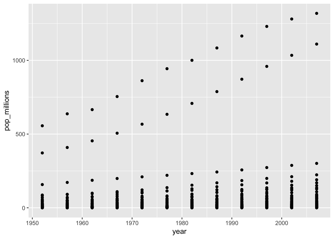
On a single graph, plot population, in millions, against year, for all countries. Don’t worry about identifying which country is which.
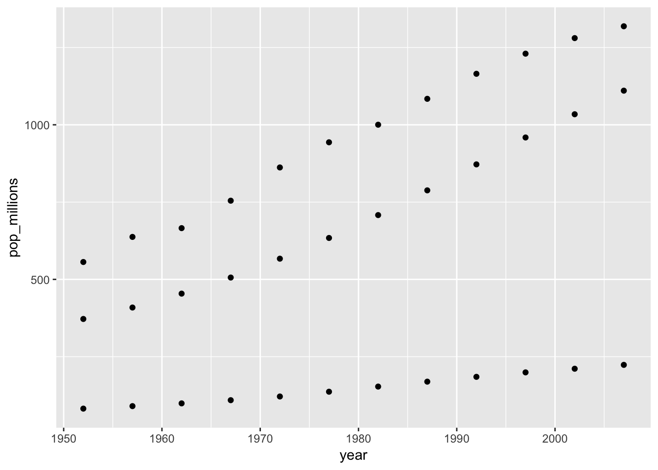
Repeat the exercise, graphing only for China, India, and Indonesia. Again, don’t worry about which is which.
Solution to challenge 2
Refresh your plotting skills by plotting population in millions against year.
ggplot(gapminder, aes(x = year, y = pop_millions)) +
 geom_point()
countryset <- c("China","India","Indonesia")
ggplot(gapminder[gapminder$country %in% countryset,],
       aes(x = year, y = pop_millions)) +
  geom_point()
Comparison operators, logical operators, and many functions are also vectorized:
Comparison operators
x > 2
## [1] FALSE FALSE TRUE TRUE
Logical operators
a <- x > 3  # or, for clarity, a <- (x > 3)
a
## [1] FALSE FALSE FALSE TRUE
Tip: some useful functions for logical vectors
any()will returnTRUEif any element of a vector isTRUEall()will returnTRUEif all elements of a vector areTRUE
Most functions also operate element-wise on vectors:
Functions
x <- 1:4
log(x)
## [1] 0.0000000 0.6931472 1.0986123 1.3862944
Vectorized operations work element-wise on matrices:
m <- matrix(1:12, nrow=3, ncol=4)
m * -1
##      [,1] [,2] [,3] [,4]
## [1,]   -1   -4   -7  -10
## [2,]   -2   -5   -8  -11
## [3,]   -3   -6   -9  -12
Tip: element-wise vs. matrix multiplication
Very important: the operator
*gives you element-wise multiplication! To do matrix multiplication, we need to use the%*%operator:m %*% matrix(1, nrow=4, ncol=1)## [,1] ## [1,] 22 ## [2,] 26 ## [3,] 30matrix(1:4, nrow=1) %*% matrix(1:4, ncol=1)## [,1] ## [1,] 30For more on matrix algebra, see the Quick-R reference guide
Challenge 3
Given the following matrix:
m <- matrix(1:12, nrow=3, ncol=4)
m
## [,1] [,2] [,3] [,4] ## [1,] 1 4 7 10 ## [2,] 2 5 8 11 ## [3,] 3 6 9 12Write down what you think will happen when you run:
m ^ -1m * c(1, 0, -1)m > c(0, 20)m * c(1, 0, -1, 2)Did you get the output you expected? If not, ask a helper!
Solution to challenge 3
Given the following matrix:
m <- matrix(1:12, nrow=3, ncol=4)
m
## [,1] [,2] [,3] [,4] ## [1,] 1 4 7 10 ## [2,] 2 5 8 11 ## [3,] 3 6 9 12Write down what you think will happen when you run:
m ^ -1## [,1] [,2] [,3] [,4] ## [1,] 1.0000000 0.2500000 0.1428571 0.10000000 ## [2,] 0.5000000 0.2000000 0.1250000 0.09090909 ## [3,] 0.3333333 0.1666667 0.1111111 0.08333333
m * c(1, 0, -1)## [,1] [,2] [,3] [,4] ## [1,] 1 4 7 10 ## [2,] 0 0 0 0 ## [3,] -3 -6 -9 -12
m > c(0, 20)## [,1] [,2] [,3] [,4] ## [1,] TRUE FALSE TRUE FALSE ## [2,] FALSE TRUE FALSE TRUE ## [3,] TRUE FALSE TRUE FALSE
Challenge 4
We’re interested in looking at the sum of the following sequence of fractions:
x = 1/(1^2) + 1/(2^2) + 1/(3^2) + ... + 1/(n^2)This would be tedious to type out, and impossible for high values of n. Use vectorisation to compute x when n=100. What is the sum when n=10,000?
Challenge 4
We’re interested in looking at the sum of the following sequence of fractions:
x = 1/(1^2) + 1/(2^2) + 1/(3^2) + ... + 1/(n^2)This would be tedious to type out, and impossible for high values of n. Can you use vectorisation to compute x, when n=100? How about when n=10,000?
sum(1/(1:100)^2)## [1] 1.634984sum(1/(1:1e04)^2)## [1] 1.644834n <- 10000 sum(1/(1:n)^2)## [1] 1.644834We can also obtain the same results using a function:
inverse_sum_of_squares <- function(n) {
  sum(1/(1:n)^2)
}
inverse_sum_of_squares(100)
## [1] 1.634984inverse_sum_of_squares(10000)## [1] 1.644834n <- 10000 inverse_sum_of_squares(n)## [1] 1.644834
Key Points
Use vectorized operations instead of loops.