Split-Apply-Combine

Overview

Teaching: 30 min
Exercises: 30 min

Questions

How can I do different calculations on different sets of data?

Objectives

To be able to use the split-apply-combine strategy for data analysis.

Previously we looked at how you can use functions to simplify your code. We defined the calcGDP function, which takes the gapminder dataset, and multiplies the population and GDP per capita column. We also defined additional arguments so we could filter by year and country:

# Takes a dataset and multiplies the population column
# with the GDP per capita column.
calcGDP <- function(dat, year=NULL, country=NULL) {
  if(!is.null(year)) {
    dat <- dat[dat$year %in% year, ]
  }
  if (!is.null(country)) {
    dat <- dat[dat$country %in% country,]
  }
  gdp <- dat$pop * dat$gdpPercap

  new <- cbind(dat, gdp=gdp)
  return(new)
}

A common task you’ll encounter when working with data, is that you’ll want to run calculations on different groups within the data. In the above, we were simply calculating the GDP by multiplying two columns together. But what if we wanted to calculated the mean GDP per continent?

We could run calcGPD and then take the mean of each continent:

withGDP <- calcGDP(gapminder)
mean(withGDP[withGDP$continent == "Africa", "gdp"])

## [1] 20904782844

mean(withGDP[withGDP$continent == "Americas", "gdp"])

## [1] 379262350210

mean(withGDP[withGDP$continent == "Asia", "gdp"])

## [1] 227233738153

But this isn’t very nice. Yes, by using a function, you have reduced a substantial amount of repetition. That is nice. But there is still repetition. Repeating yourself will cost you time, both now and later, and potentially introduce some nasty bugs.

We could write a new function that is flexible like calcGDP, but this also takes a substantial amount of effort and testing to get right.

The abstract problem we’re encountering here is know as “split-apply-combine”:

Split apply combine

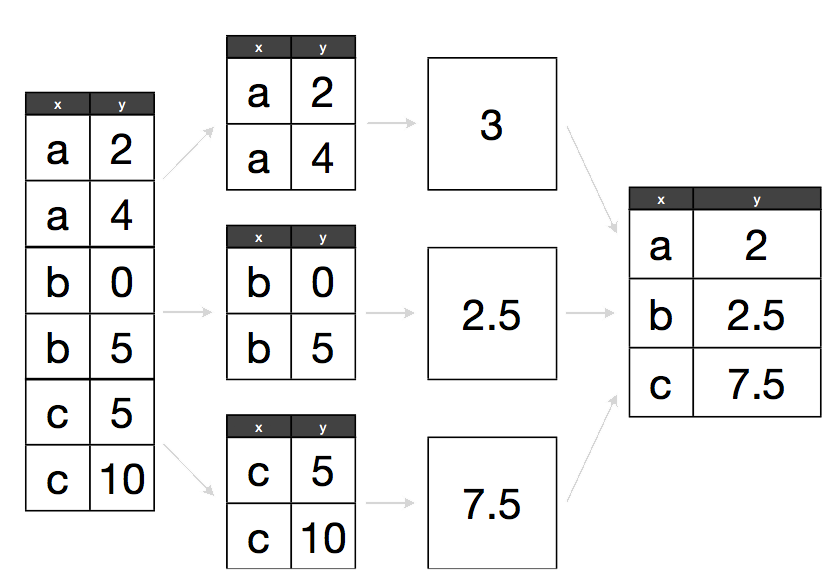
We want to split our data into groups, in this case continents, apply some calculations on that group, then optionally combine the results together afterwards.

The `plyr` package

For those of you who have used R before, you might be familiar with the apply family of functions. While R’s built in functions do work, we’re going to introduce you to another method for solving the “split-apply-combine” problem. The plyr package provides a set of functions that we find more user friendly for solving this problem.

We installed this package in an earlier challenge. Let’s load it now:

library(plyr)

Plyr has functions for operating on lists, data.frames and arrays (matrices, or n-dimensional vectors). Each function performs:

A splitting operation
Apply a function on each split in turn.
Recombine output data as a single data object.

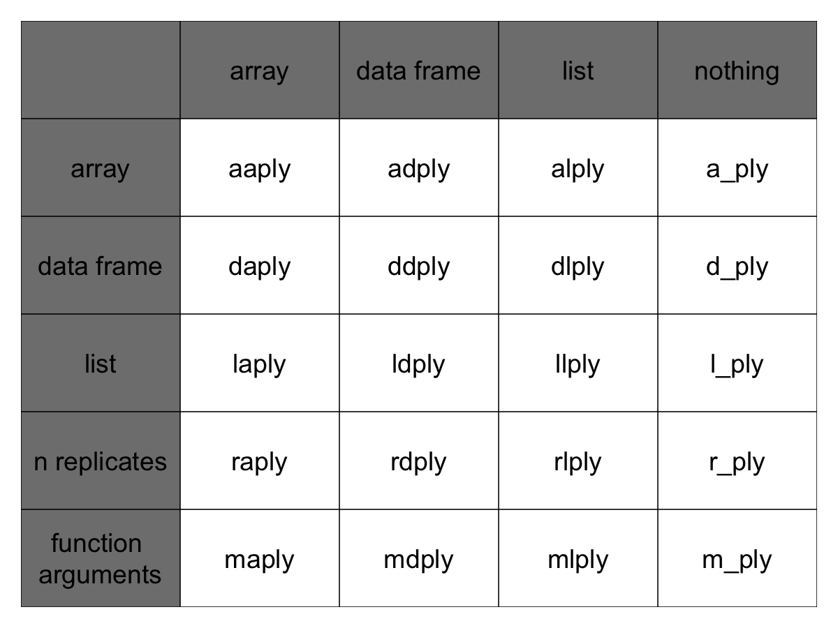
The functions are named based on the data structure they expect as input, and the data structure you want returned as output: [a]rray, [l]ist, or [d]ata.frame. The first letter corresponds to the input data structure, the second letter to the output data structure, and then the rest of the function is named “ply”.

This gives us 9 core functions **ply. There are an additional three functions which will only perform the split and apply steps, and not any combine step. They’re named by their input data type and represent null output by a _ (see table)

Note here that plyr’s use of “array” is different to R’s, an array in ply can include a vector or matrix.

Full apply suite

Each of the xxply functions (daply, ddply, llply, laply, …) has the same structure and has 4 key features and structure:

xxply(.data, .variables, .fun)

The first letter of the function name gives the input type and the second gives the output type.
.data - gives the data object to be processed
.variables - identifies the splitting variables
.fun - gives the function to be called on each piece

Now we can quickly calculate the mean GDP per continent:

ddply(
 .data = calcGDP(gapminder),
 .variables = "continent",
 .fun = function(x) mean(x$gdp)
)

##   continent           V1
## 1    Africa  20904782844
## 2  Americas 379262350210
## 3      Asia 227233738153
## 4    Europe 269442085301
## 5   Oceania 188187105354

Let’s walk through the previous code:

The ddply function feeds in a data.frame (function starts with d) and returns another data.frame (2nd letter is a d) i
the first argument we gave was the data.frame we wanted to operate on: in this case the gapminder data. We called calcGDP on it first so that it would have the additional gdp column added to it.
The second argument indicated our split criteria: in this case the “continent” column. Note that we gave the name of the column, not the values of the column like we had done previously with subsetting. Plyr takes care of these implementation details for you.
The third argument is the function we want to apply to each grouping of the data. We had to define our own short function here: each subset of the data gets stored in x, the first argument of our function. This is an anonymous function: we haven’t defined it elsewhere, and it has no name. It only exists in the scope of our call to ddply.

What if we want a different type of output data structure?:

dlply(
 .data = calcGDP(gapminder),
 .variables = "continent",
 .fun = function(x) mean(x$gdp)
)

## $Africa
## [1] 20904782844
## 
## $Americas
## [1] 379262350210
## 
## $Asia
## [1] 227233738153
## 
## $Europe
## [1] 269442085301
## 
## $Oceania
## [1] 188187105354
## 
## attr(,"split_type")
## [1] "data.frame"
## attr(,"split_labels")
##   continent
## 1    Africa
## 2  Americas
## 3      Asia
## 4    Europe
## 5   Oceania

We called the same function again, but changed the second letter to an l, so the output was returned as a list.

We can specify multiple columns to group by:

ddply(
 .data = calcGDP(gapminder),
 .variables = c("continent", "year"),
 .fun = function(x) mean(x$gdp)
)

##    continent year           V1
## 1     Africa 1952   5992294608
## 2     Africa 1957   7359188796
## 3     Africa 1962   8784876958
## 4     Africa 1967  11443994101
## 5     Africa 1972  15072241974
## 6     Africa 1977  18694898732
## 7     Africa 1982  22040401045
## 8     Africa 1987  24107264108
## 9     Africa 1992  26256977719
## 10    Africa 1997  30023173824
## 11    Africa 2002  35303511424
## 12    Africa 2007  45778570846
## 13  Americas 1952 117738997171
## 14  Americas 1957 140817061264
## 15  Americas 1962 169153069442
## 16  Americas 1967 217867530844
## 17  Americas 1972 268159178814
## 18  Americas 1977 324085389022
## 19  Americas 1982 363314008350
## 20  Americas 1987 439447790357
## 21  Americas 1992 489899820623
## 22  Americas 1997 582693307146
## 23  Americas 2002 661248623419
## 24  Americas 2007 776723426068
## 25      Asia 1952  34095762654
## 26      Asia 1957  47267432088
## 27      Asia 1962  60136869012
## 28      Asia 1967  84648519224
## 29      Asia 1972 124385747313
## 30      Asia 1977 159802590186
## 31      Asia 1982 194429049919
## 32      Asia 1987 241784763369
## 33      Asia 1992 307100497486
## 34      Asia 1997 387597655323
## 35      Asia 2002 458042336179
## 36      Asia 2007 627513635079
## 37    Europe 1952  84971341466
## 38    Europe 1957 109989505140
## 39    Europe 1962 138984693095
## 40    Europe 1967 173366641137
## 41    Europe 1972 218691462733
## 42    Europe 1977 255367522034
## 43    Europe 1982 279484077072
## 44    Europe 1987 316507473546
## 45    Europe 1992 342703247405
## 46    Europe 1997 383606933833
## 47    Europe 2002 436448815097
## 48    Europe 2007 493183311052
## 49   Oceania 1952  54157223944
## 50   Oceania 1957  66826828013
## 51   Oceania 1962  82336453245
## 52   Oceania 1967 105958863585
## 53   Oceania 1972 134112109227
## 54   Oceania 1977 154707711162
## 55   Oceania 1982 176177151380
## 56   Oceania 1987 209451563998
## 57   Oceania 1992 236319179826
## 58   Oceania 1997 289304255183
## 59   Oceania 2002 345236880176
## 60   Oceania 2007 403657044512

daply(
 .data = calcGDP(gapminder),
 .variables = c("continent", "year"),
 .fun = function(x) mean(x$gdp)
)

##           year
## continent          1952         1957         1962         1967
##   Africa     5992294608   7359188796   8784876958  11443994101
##   Americas 117738997171 140817061264 169153069442 217867530844
##   Asia      34095762654  47267432088  60136869012  84648519224
##   Europe    84971341466 109989505140 138984693095 173366641137
##   Oceania   54157223944  66826828013  82336453245 105958863585
##           year
## continent          1972         1977         1982         1987
##   Africa    15072241974  18694898732  22040401045  24107264108
##   Americas 268159178814 324085389022 363314008350 439447790357
##   Asia     124385747313 159802590186 194429049919 241784763369
##   Europe   218691462733 255367522034 279484077072 316507473546
##   Oceania  134112109227 154707711162 176177151380 209451563998
##           year
## continent          1992         1997         2002         2007
##   Africa    26256977719  30023173824  35303511424  45778570846
##   Americas 489899820623 582693307146 661248623419 776723426068
##   Asia     307100497486 387597655323 458042336179 627513635079
##   Europe   342703247405 383606933833 436448815097 493183311052
##   Oceania  236319179826 289304255183 345236880176 403657044512

You can use these functions in place of for loops (and its usually faster to do so). To replace a for loop, put the code that was in the body of the for loop inside an anonymous function.

d_ply(
  .data=gapminder,
  .variables = "continent",
  .fun = function(x) {
    meanGDPperCap <- mean(x$gdpPercap)
    print(paste(
      "The mean GDP per capita for", unique(x$continent),
      "is", format(meanGDPperCap, big.mark=",")
   ))
  }
)

## [1] "The mean GDP per capita for Africa is 2,193.755"
## [1] "The mean GDP per capita for Americas is 7,136.11"
## [1] "The mean GDP per capita for Asia is 7,902.15"
## [1] "The mean GDP per capita for Europe is 14,469.48"
## [1] "The mean GDP per capita for Oceania is 18,621.61"

Tip: printing numbers

The format function can be used to make numeric values “pretty” for printing out in messages.

Challenge 1

Calculate the average life expectancy per continent. Which has the longest? Which had the shortest?

Challenge 2

Calculate the average life expectancy per continent and year. Which had the longest and shortest in 2007? Which had the greatest change in between 1952 and 2007?

Advanced Challenge

Calculate the difference in mean life expectancy between the years 1952 and 2007 from the output of challenge 2 using one of the plyr functions.

Alternate Challenge if class seems lost

Without running them, which of the following will calculate the average life expectancy per continent:

ddply(
  .data = gapminder,
  .variables = gapminder$continent,
  .fun = function(dataGroup) {
     mean(dataGroup$lifeExp)
  }
)

ddply(
  .data = gapminder,
  .variables = "continent",
  .fun = mean(dataGroup$lifeExp)
)

ddply(
  .data = gapminder,
  .variables = "continent",
  .fun = function(dataGroup) {
     mean(dataGroup$lifeExp)
  }
)

adply(
  .data = gapminder,
  .variables = "continent",
  .fun = function(dataGroup) {
     mean(dataGroup$lifeExp)
  }
)

Key Points

Use the plyr package to split data, apply functions to subsets, and combine the results.

previous episode

R for Reproducible Research

next episode

Split-Apply-Combine

Overview

The `plyr` package

Tip: printing numbers

Challenge 1

Challenge 2

Advanced Challenge

Alternate Challenge if class seems lost

Key Points

previous episode

next episode